Want to understand the average size of hidden representations?

You should! This is foundational for understanding everything else about the dynamics of neural networks.

Historically, the first questions people tried to answer about neural networks dealt with their performance and representations: how can we characterize how well our network performs, and what hidden representations do they learn as they train? We’ll revisit these questions later in a modern light, but suffice it to say that they are hard and it’s unclear where to start. In rigorous science, it’s usually a good idea to be humble about what you can understand and to start with the dumbest, simplest question you think you can answer, working up from there. It turns out that the simplest useful theoretical question you can ask about neural networks is: as you forward-propagate your signal and backprop your gradient, roughly how big are the (pre)activations and gradients on average? Answering this is useful for understanding initialization, avoiding exploding or vanishing gradients, and getting stable optimization even in large models.

More precisely: suppose we have an input vector \(\mathbf{x}\) (an image, token, set of features, etc.), and we start propagating forward through our network, stopping part way. Denote by \(\mathbf{h}_\ell(\mathbf{x})\) the hidden representations after applying the \(\ell\)-th linear layer. What’s the typical size of an element of \(\mathbf{h}_\ell(\mathbf{x})\)? If you want a mathematical metric for this, you might study the root-mean-squared size

\[ q_\ell(\mathbf{x}) := \frac{|\!|{\mathbf{h}_\ell(\mathbf{x})}|\!|}{\sqrt{\text{size}[\mathbf{h}_\ell(\mathbf{x})]}}. \]

You don’t want \(q_\ell(\mathbf{x})\) to either blow up or vanish as you propagate forwards through the network. If either happens, you’ll be feeding very large or very small arguments to your activation function,¹ which is generally a bad idea.² In a neural network of many layers, problems like this tend to get worse as you propagate through more and more layers, so you want to avoid them from the get go.

First steps: LeCun initialization and large width

The first people to address this question seriously were practitioners in the 1990s. If you initialize a neural network’s weight parameters with unit variance — that is, \(W_{ij} \sim \mathcal{N}(0,1)\) — then your preactivations tend to blow up. If instead you initialize with

\[ W_{ij} \sim \mathcal{N}(0, \sigma^2), \]

where \(\sigma^2 = \frac{1}{\text{[fan in]}}\), the preactivations are better controlled. By a central limit theorem calculation, this init size ensures that well-behaved activations in the previous layer mean well-behaved preactivations in the following layer, at least at initialization.

• This scheme is now called LeCun initialization after [LeCun et al. (1996)].

This is the first calculation any new deep learning scientist should be able to perform! Get comfortable with this kind of central limit theorem argument.

The central limit theorem gives the best approximation for a sum as the number of added terms grows. This suggests that, when studying any sort of signal propagation problem, it’s a good and useful idea to consider the case of large width. This is the consideration that motivates the study of infinite-width networks, which are now central in the mathematical science of deep learning. It’s very important to think about this enough to have intuition for why the large-width limit is useful.

Infinite-width nets at init: signal propagation and the neural network Gaussian process (NNGP)

A natural next question is: what else can you say about wide neural networks at initialization? The answer unfolds in the following sequence.

First, you can perform a close study of the “signal sizes” \(q_\ell(\mathbf{x})\) as well as the correlations \(c_\ell(\mathbf{x}, \mathbf{x}') := \langle \mathbf{h}_\ell(\mathbf{x}), \mathbf{h}_\ell(\mathbf{x}') \rangle\). You can actually calculate both of these exactly at infinite width using Gaussian integrals.

• See [Poole et al. (2016)] for a derivation physicists will like and [Daniely et al. (2016)] for a more formal treatment better suited for mathematicians.
  • It’s worth getting to the point where you understand either Eqns (1-5) from [Poole et al. (2016)] or Sections 5 and 8 from [Daniely et al. (2016)]. The other stuff — chaos, computational graphs, and so on — is cool but not essential.
• See [Schoenholz et al. (2016)] for a similar size analysis for the backpropagated gradients.

Next, you can study not only the averages of these quantities but also their complete distributions. It turns out they’re Gaussian at initialization (surprise, surprise) and the network function value itself is a “Gaussian process” with a covariance kernel that you can obtain in closed form.

• This was first worked out for shallow networks by [Neal (1996)]. It took another two decades before it was extended to deep networks by [Lee et al. (2017)]. If you train only the last layer of a wide neural network, the resulting learning rule is equivalent to Gaussian process regression with the NNGP.

It’s very worth working through the NNGP idea and getting intuition for both GPs and the forward-prop statistics that give a GP in this context. Notice that MLPs have NNGPs with rotation-invariant kernels. This will remain a useful intuition.

At this point in our discussion, we already have papers that have calculated average-case quantities exactly which agree well with experiments using networks with widths in the hundreds or thousands. Look at how good the agreement is in these plots:

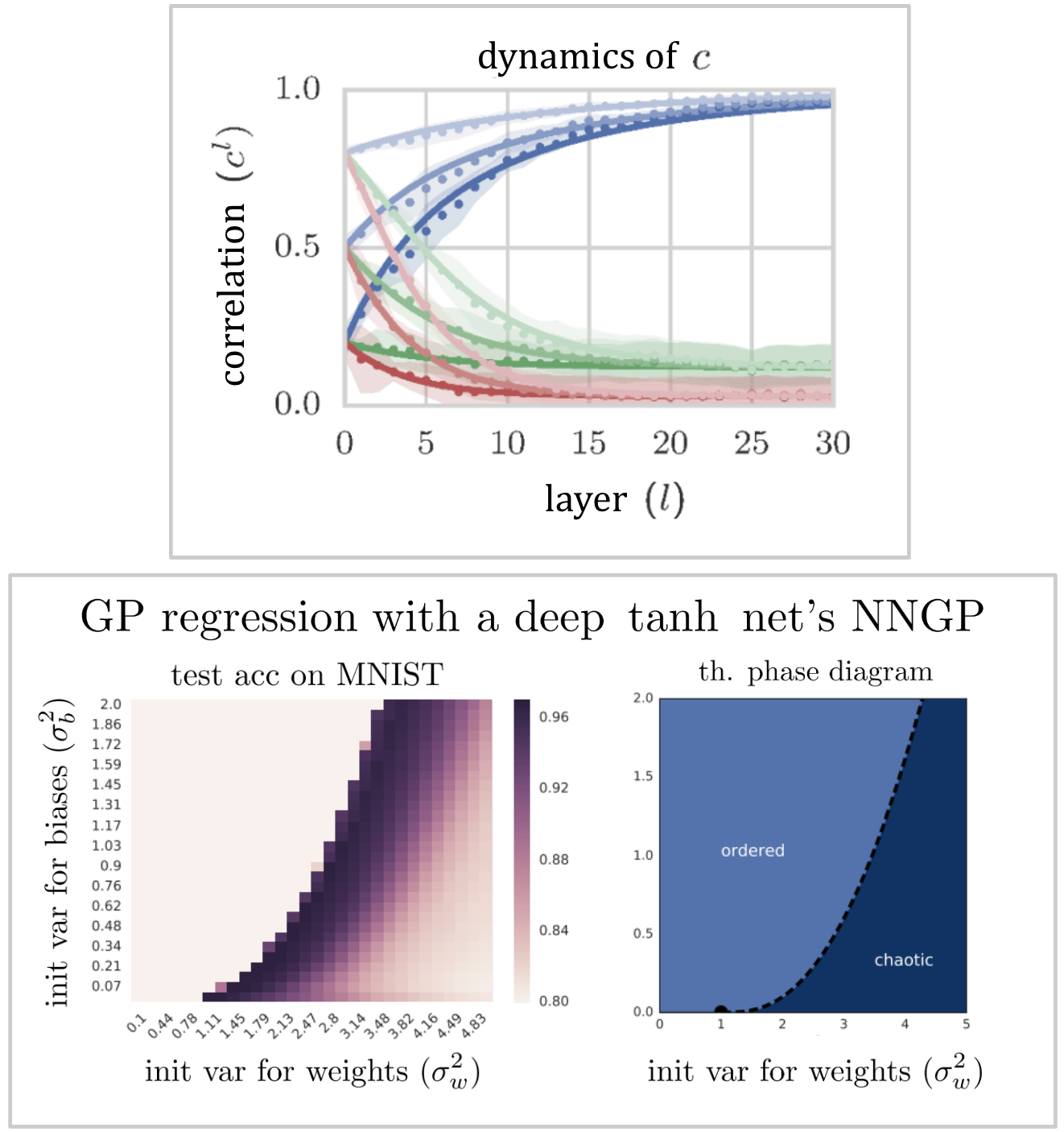
Top: signal propagation of layerwise correlations for a deep \(\tanh\) net from Poole et al. (2016). Blue, green, and red sets of curves correspond to weight initialization variances \(\sigma_w^2 = \{1.3, 2.3, 4.0\}\). Different saturations correspond to different initial correlations. Experiment dots lie very close to the theory curves. Bottom: performance of NNGP regression vs. ordered/chaotic regimes from Lee et al. (2017). Left subplot shows the test accuracy of GP regression with a depth-50 \(\tanh\) NNGP on MNIST. Right subplot shows prediction of the ordered and chaotic regimes using the same machinery as Poole et al. (2016). The best performance falls near the boundary between order and chaos. It’s significant that we can quantitatively predict the structure of a phase diagram of model performance, even in a simplified setting like NNGP regression.

It’s worth appreciating that extremely good agreement with experiment is possible if we’re studying the right objects in the right regimes. Most deep learning theory work that can’t get agreement this good eventually fades or is replaced by something that does. It’s usually wise to insist on a quantitative match from your theory and be satisfied with nothing less.

Infinite-width nets under gradient descent: the NTK

Now that we understand initialization in wide networks, we’re ready to study training. The first milestone on this path is the “neural tangent kernel” (NTK). The main result here is that if you train a neural network in the NNGP infinite-width setting, its functional evolution is described by a particular kernel which remains static for all time. This kernel is the inner product of parameter gradient vectors:

\[ \text{NTK}(\mathbf{x}, \mathbf{x}') := \left\langle \nabla_{\boldsymbol{\theta}} f_{\boldsymbol{\theta}}(\mathbf{x}), \nabla_{\boldsymbol{\theta}} f_{\boldsymbol{\theta}}(\mathbf{x}') \right\rangle. \]

The primary consequence is that, in this limit, the learning dynamics of a neural networks is, by the “kernel trick,” equivalent to the dynamics of a linear model. The final learned function is given by kernel (ridge) regression.

• The original NTK paper is that of [Jacot et al. (2018)]. The subsequent presentation of [Lee et al. (2019)] is less formal and may be easier for beginners.
  • The NTK idea is a bit too technical to explain here (though we sure want to), but it’s all but essential to understand it before moving on to feature learning. It’s worth allocating some time, working through one of these papers, and making sure you’ve extracted the simple core idea. It’s also worth thinking carefully about linear models and kernel regression, as these will return later as first models for other learning phenomena.
  • Notice that one can make accurate quantitative predictions for the learning of wide nets using the NTK. See, for example, Figure 2 of [Lee et al. (2019)].

Motivated by the NTK, people found new and clever ways to ask and answer for kernel regression the questions we want answered of deep learning. This gave the field a useful new tool and has led to some moderately valuable insights. For example, networks in the NTK limit always converge to zero training loss so long as the learning rate isn’t too big, and this served as a useful demonstration of how overparameterization usually makes optimization easier, not harder. Kernel models will appear a few other times in other chapters of this guide.

Scaling analysis of feature evolution: the maximal update parameterization (\(\mu\)P)

After the development of the NTK, people quickly noticed that networks in this limit don’t exhibit feature learning. That is, at infinite width, the hidden neurons of a network represent the same functions after training as they did at initialization. At large-but-finite width, the change is finite but negligible. This is a first clue that the pretty, analytically tractable NTK limit isn’t the end of the story.³

For a few years, it seemed like we might have to give up on infinite-width networks. Fortunately, it turned out that there’s another coherent infinite-width limit in which things scale differently, and the network does actually undergo feature learning. This is the regime in which most deep learning theory now takes place.

Here’s the evolution of ideas, some key papers, and key takeaways:

• [Chizat and Bach (2018)] gave a “lazy” vs. “rich” dichotomy of gradient descent dynamics, using “lazy” to mean “kernel dynamics” and “rich” to mean “anything else.”
  • It’s worth understanding what “lazy” training is, and how an output multiplier can make any neural network train lazily.
• [Mei et al (2018)], [Rotskoff and Vanden-Eijnden (2018)], and a handful of other authors pointed out a “mean-field” parameterization that allows infinite-width shallow neural nets to learn features. They give it different names but describe the same parameterization.
  • This may be an easier place to start than \(\mu\)P, but if you understand \(\mu\)P, you can skip mean-field nets for now.
• [Yang and Hu (2021)] extended this insight to deep networks. They pointed out a way that layerwise init sizes + learning rates can scale with network width so that a deep network learns features to leading order even at infinite width. They call this the “maximal update parameterization” (muP, or \(\mu\)P).
  • The core idea here is extremely important and can be understood in simple terms. Their “Tensor Programs” and “abc-param” frameworks are fairly complicated — you don’t need to understand either to get the main gist. [Yang et al. (2023)] give a simpler framing of the big idea here, and [Karkada (2024)] give a beginner-friendly tutorial of the NTK/\(\mu\)P story.
• [Yang et al. (2022)] showed that this parameterization is practically useful: it lets one scale up neural networks while preserving network hyperparameters. (More on this in our discussion of hyperparameters.)
  • This is probably the first practically impactful achievement of deep learning theory in the modern era, so it’s worth thinking about seriously.

These “rich,” feature learning, \(\mu\)P dynamics led to a paradigm shift in deep learning theory. Most later work uses or relates to it in some way. It’s thus very important to understand. A seasoned deep learning theorist should be able to sit down and derive the \(\mu\)P parameterization, or something equivalent to it, from first principles. It’s difficult to do relevant work in 2025 without it!

It’s worth noting that, unlike the NTK limit, the \(\mu\)P limit is very difficult to study analytically. In the NTK limit, we have kernel behavior, simple gradient descent dynamics, a convex loss surface (using squared loss), and lots of older theoretical tools that we can bring to bear. In the \(\mu\)P limit, we have none of this. To our knowledge, nobody’s even shown a general result that a deep network in the \(\mu\)P limit converges, let alone characterized the solution that’s found!

In the NTK limit, we can study the model with the well-established math of kernel theory, which already existed and has now been developed further expressly for the study of the NTK. In the \(\mu\)P limit, the best we have so far are rather complex calculational frameworks:

• The dynamical mean-field theory (DMFT) frameworks of [Bordelon and Pehlevan (2022)] and [Dandi et al. (2024)] let one compute feature distributions of infinite-width networks in the rich regime, but it is quite complicated, and it is difficult to extract analytical insight. (It is nonetheless useful for scaling calculations.) The Tensor Programs framework of [Yang and Hu (2021)] allows one to perform the same calculations with random matrix theory language.
  • These are specialized tools and are not essential on a first pass through deep learning theory.

Onwards: towards infinite depth

Early in this chapter, we took width to infinity, which allowed us a host of useful calculational tools. We can also take depth to infinity. There are several ways to do this, but the upshot is that one quickly encounters stability problems with a standard MLP, so a ResNet formulation in which each layer gets a small premultiplier seems like the most promising choice.

• [Bordelon et al. (2023)] and [Yang et al. (2023)] give treatments of \(\mu\)P at large depth. They conclude with slightly different scaling recommendations for layerwise premultipliers.
  • This is probably useful to understand for the future but is not yet essential knowledge. As with \(\mu\)P, the most important thing to get out of either paper is the scaling calculation that gives the hyperparameter prescription.